
Awesome news, pg_stat_monitor has reached a GA STATUS! Percona has long been associated with pushing the limits and understanding the nuances involved in running database systems at scale, so building a tool that helps get us there brings a bit more insight and details around query performance and scale on PostgreSQL systems fits with our history. So what the hell does pg_stat_monitor do, and why should you care? Excellent question!
Currently, for collecting and reviewing query metrics, the defacto standard is pg_stat_statements. This extension collects query metrics and allows you to go back and see which queries have impacted your system. Querying the extension would yield something like this:
|
1 2 3 4 5 6 7 8 9 10 11 12 13 14 15 16 17 18 19 20 21 22 23 24 25 26 27 28 29 30 31 32 33 34 35 36 37 38 39 40 41 42 43 44 45 46 47 48 49 50 51 52 |
postgres=# dx List of installed extensions -[ RECORD 1 ]----------------------------------------------------------------------- Name | pg_stat_statements Version | 1.8 Schema | public Description | track planning and execution statistics of all SQL statements executed -[ RECORD 2 ]----------------------------------------------------------------------- Name | plpgsql Version | 1.0 Schema | pg_catalog Description | PL/pgSQL procedural language postgres=# x Expanded display is on. postgres=# select * from pg_stat_statements; -[ RECORD 2 ]-------+-------------------------------------------------------- userid | 16384 dbid | 16608 queryid | -7945632213382375966 query | select ai_myid, imdb_id, year, title, json_column from movies_normalized_meta where ai_myid = $1 plans | 0 total_plan_time | 0 min_plan_time | 0 max_plan_time | 0 mean_plan_time | 0 stddev_plan_time | 0 calls | 61559 total_exec_time | 27326.783784999938 min_exec_time | 0.062153 max_exec_time | 268.55287599999997 mean_exec_time | 0.44391208084927075 stddev_exec_time | 2.522740928486301 rows | 61559 shared_blks_hit | 719441 shared_blks_read | 1031 shared_blks_dirtied | 0 shared_blks_written | 0 local_blks_hit | 0 local_blks_read | 0 local_blks_dirtied | 0 local_blks_written | 0 temp_blks_read | 0 temp_blks_written | 0 blk_read_time | 0 blk_write_time | 0 wal_records | 6 wal_fpi | 0 wal_bytes | 336 |
You can see here that this particular statement has been executed 61,559 times, and had a total time taken of 27,326 Milliseconds, for a mean time of 0.44 MS.
You can also get metrics on if this statement is writing data, generating wal, etc. This is valuable to help find what statement may be missing cache and hitting disk, or which statements may be blowing up your wal logs.
While this data is great, it could be better. Specifically, it’s hard to determine if problems are getting worse or better. Also, what if that particular query that executed 61K times runs in .01ms 60K times and 1000 ms 1K times. Collecting enough data here to make better, more targeted decisions around optimization is needed. This is where pg_stat_monitor can help.
First let me show you the output from one of the collected queries (note I am only selecting a single bucket, more on that in a second):
|
1 2 3 4 5 6 7 8 9 10 11 12 13 14 15 16 17 18 19 20 21 22 23 24 25 26 27 28 29 30 31 32 33 34 35 36 37 38 39 40 41 42 43 44 45 46 47 48 49 50 51 52 53 54 55 56 57 |
postgres=# postgres=# x Expanded display is on. postgres=# select * from pg_stat_monitor ; -[ RECORD 1 ]-------+--------- bucket | 3 bucket_start_time | 2022-04-27 20:13:00 userid | movie_json_user datname | movie_json_test client_ip | 172.31.33.208 queryid | 82650C255980E05 top_queryid | query | select ai_myid, imdb_id, year, title, json_column from movies_normalized_meta where ai_myid = $1 comments | planid | query_plan | top_query | application_name | relations | {public.movies_normalized_meta} cmd_type | 1 cmd_type_text | SELECT elevel | 0 sqlcode | message | calls | 18636 total_exec_time | 9022.0356 min_exec_time | 0.055 max_exec_time | 60.7575 mean_exec_time | 0.4841 stddev_exec_time | 1.568 rows_retrieved | 18636 plans_calls | 0 total_plan_time | 0 min_plan_time | 0 max_plan_time | 0 mean_plan_time | 0 stddev_plan_time | 0 shared_blks_hit | 215919 shared_blks_read | 1 shared_blks_dirtied | 39 shared_blks_written | 0 local_blks_hit | 0 local_blks_read | 0 local_blks_dirtied | 0 local_blks_written | 0 temp_blks_read | 0 temp_blks_written | 0 blk_read_time | 0 blk_write_time | 0 resp_calls | {17946,629,55,6,0,0,0,0,0,0} cpu_user_time | 3168.0737 cpu_sys_time | 1673.599 wal_records | 9 wal_fpi | 0 wal_bytes | 528 state_code | 3 state | FINISHED |
You can see there is a lot of extra data. Let’s view these side by side:
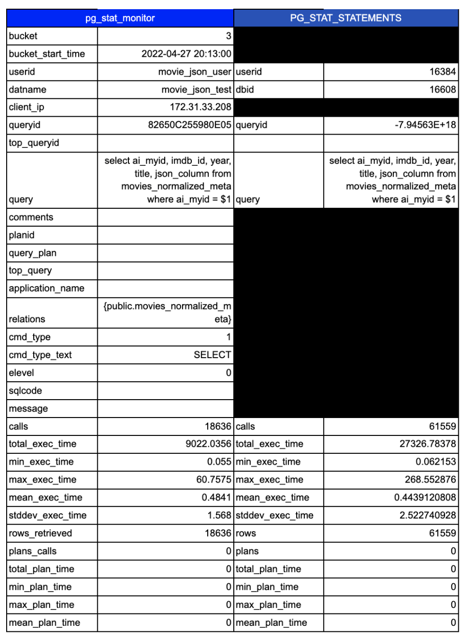
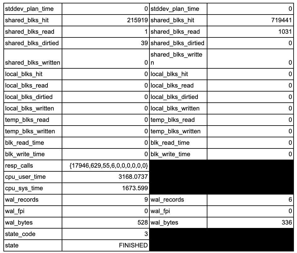
There are 19 additional columns of collected data. Some of that extra data is used to break down the data into more granular and useful views of the data.
First up is the introduction of the concept of “buckets”. What are buckets? This is a configurable slice of time. Instead of everything stored in a single big bucket, you can now add the ability to break query stats into timed buckets that allow you to look at performance changes for a query over a time period. Note these default to a max of 10 buckets each containing 60 seconds of data (this is configurable). This means the query data is easily consumable by your favorite time-series database for even more historical analysis capabilities. We use these buckets internally to pull data into our query analytics tool and store them in a click house time-series database to provide even more analytic capabilities.
Note the difference between pg_stat_statement and pg_stat_monitor with regard to data retention. Pg_stat_monitor is best used in conjunction with another monitoring tool if you need long-term storage of query data.
Next, you will notice the inclusion of user/connection details. Many applications use the same user, but have several endpoints connecting. Breaking up data via the client IP helps track down that rogue user or application server causing issues.
You can get a full breakdown of the features, settings, and columns here in the docs: https://percona.github.io/pg_stat_monitor/REL1_0_STABLE/USER_GUIDE.html
But I want to highlight a few of the new metrics and capabilities I am most excited about. For me, the most interesting is the ability to collect histogram data. This enables you to see if queries that deviate from the normal. One of the key things our support engineers are always looking at is how is the P99 latency, and this helps with that. You can see Percona Monitoring and Management take advantage of these features here:
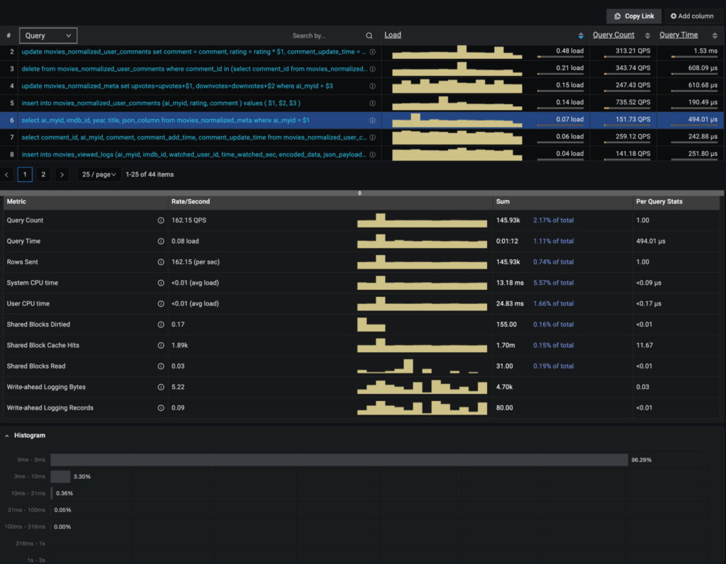
With the histograms enabled, I can see and help track down where queries and performance deviate from the normal.
Additionally, you will notice the inclusion of CPU time. Why is this important? Query timings include things like waiting on disk and network resources. If you have a system with a CPU bottleneck, the queries taking the longest time may or may not be the offender.
Finally, you can configure pg_stat_monitor to store explain plans from previously run queries. This is incredibly useful when plans change over time, and you are trying to recreate what took place an hour or two ago.
Gaining additional insights and understanding your workload is critical, and pg_stat_monitor can help you do both. pg_stat_monitor enables end-to-end traceability, aggregated stats across configurable time windows, and query-wise execution time, but it is PMM that visualizes this and lets the user get even more insight into PostgreSQL behavior.
Want to try this out for yourself? The instructions are available here: https://percona.github.io/pg_stat_monitor/REL1_0_STABLE/setup.html#installing-from-percona-repositories
Also, check out the video walkthrough where I installed the plugin:
Resources
RELATED POSTS


While this tool has high expectations in taking pg_stat_statements to the next level, support for this tool is not very good.
I created a critical bug with them 2 weeks ago that is not being addressed. It is just marked as TO BE DONE IN THE NEXT SPRINT. This bug will crash the PostgreSQL Instance –> https://jira.percona.com/browse/PG-382.
How can you all tout this is going GA soon when you have critical outstanding bugs like this that are not being addressed? Not very impressed with the support team for this product. I will caution my clients to not use it due to is critical instability.
It looks like the engineering team is engaged with you on Jira on this. Apologies for the delayed response. We are actively looking into it.
Hi, thanks for article, it looks really helpful for observability.
How much overhead pg_stat_monitor brings to execution times of queries?
Hi Kirill,
as we speak, there is another fresh benchmark running against our GA release. As soon as those runs are through I’ll post an update.
Hi, thanks for this tool! Did you get an idea of how much overhead this extension adds in your benchmarks?