Where the open source database community meets: Use code PERCONA75 and secure your spot for Percona Live. Register

Downloads

Blog

Introducing PostgreSQL 15: Working with SELECT DISTINCT

July 13, 2022

Author

Robert Bernier

Insight for DBAs

PostgreSQL

Share this Post:

It is that time of year when we once again look at the newest version of PostgreSQL.

As tradition dictates here at Percona, the team is given a list of features to write about. Mine happened to be about a basic and important function: SELECT DISTINCT.

Before getting into the details, I would like to mention a couple of caveats about how the results were derived for this blog:

The tables are small and use a simple architecture.
Because this demonstration was performed on a relatively low-powered system, the real-world metrics have the potential to be significantly greater than what is demonstrated here.

What is the PostgreSQL SELECT DISTINCT Clause?

For those new to Postgres, and to the ANSI SQL standard, the SELECT DISTINCT statement eliminates duplicate rows from the result set by matching specified expressions. PostgreSQL DISTINCT keeps one row from each group of duplicates.

For example, given the following table:

table t_ex;
 c1 | c2
----+----
  2 | B
  4 | C
  6 | A
  2 | C
  4 | B
  6 | B
  2 | A
  4 | B
  6 | C
  2 | C

table t_ex;

c1 | c2

----+----

2 | B

4 | C

6 | A

2 | C

4 | B

6 | B

2 | A

4 | B

6 | C

2 | C

This SQL statement returns records by filtering unique values found in column “c1” in sorted order:

SELECT DISTINCT ON (c1) * FROM t_ex;

1	SELECT DISTINCT ON (c1) * FROM t_ex;

Notice, as indicated by column “c2”, that uniqueness on c1 returns the first value found in the table:

 c1 | c2
----+----
  2 | B
  4 | B
  6 | B

c1 | c2

----+----

2 | B

4 | B

6 | B

This SQL statement returns records by filtering unique values found in column “c2”:

SELECT DISTINCT ON (c2) * FROM t_ex;

1	SELECT DISTINCT ON (c2) * FROM t_ex;

 c1 | c2
----+----
  6 | A
  2 | B
  4 | C

c1 | c2

----+----

6 | A

2 | B

4 | C

And finally, returning uniqueness for the entire row:

SELECT DISTINCT * FROM t_ex;

1	SELECT DISTINCT * FROM t_ex;

 c1 | c2
----+----
  2 | A
  6 | B
  4 | C
  2 | B
  6 | A
  2 | C
  4 | B
  6 | C

c1 | c2

----+----

2 | A

6 | B

4 | C

2 | B

6 | A

2 | C

4 | B

6 | C

So what is the special new enhancement of DISTINCT? The answer is that it has been parallelized!

In the past, only a single CPU or process was used to count the number of distinct records. However, in Postgres 15, you can now break up the task by running multiple workers in parallel, each assigned to a separate CPU process. Several runtime parameters control this behavior, but the one we will focus on is max_parallel_workers_per_gather.

PostgreSQL DISTINCT Clause Examples: Generating Metrics

Let’s generate some metrics.

To demonstrate the improved performance, three tables were created without indexes and populated with approximately 5,000,000 records. Notice the number of columns for each table: one, five, and 10, respectively.

                 Table "public.t1"
 Column |  Type   | Collation | Nullable | Default
--------+---------+-----------+----------+---------
 c1     | integer |           |          |

Table "public.t1"

Column | Type | Collation | Nullable | Default

--------+---------+-----------+----------+---------

c1 | integer | | |

                        Table "public.t5"
 Column |         Type          | Collation | Nullable | Default
--------+-----------------------+-----------+----------+---------
 c1     | integer               |           |          |
 c2     | integer               |           |          |
 c3     | integer               |           |          |
 c4     | integer               |           |          |
 c5     | character varying(40) |           |          |

Table "public.t5"

Column | Type | Collation | Nullable | Default

--------+-----------------------+-----------+----------+---------

c1 | integer | | |

c2 | integer | | |

c3 | integer | | |

c4 | integer | | |

c5 | character varying(40) | | |

                        Table "public.t10"
 Column |         Type          | Collation | Nullable | Default
--------+-----------------------+-----------+----------+---------
 c1     | integer               |           |          |
 c2     | integer               |           |          |
 c3     | integer               |           |          |
 c4     | integer               |           |          |
 c5     | character varying(40) |           |          |
 c6     | integer               |           |          |
 c7     | integer               |           |          |
 c8     | integer               |           |          |
 c9     | integer               |           |          |
 c10    | integer               |           |          |

Table "public.t10"

Column | Type | Collation | Nullable | Default

--------+-----------------------+-----------+----------+---------

c1 | integer | | |

c2 | integer | | |

c3 | integer | | |

c4 | integer | | |

c5 | character varying(40) | | |

c6 | integer | | |

c7 | integer | | |

c8 | integer | | |

c9 | integer | | |

c10 | integer | | |

INSERT INTO t1 SELECT generate_series(1, 500);

1	INSERT INTO t1 SELECT generate_series(1, 500);

INSERT INTO t5
SELECT
    generate_series(1, 500),
    generate_series(500, 1000),
    generate_series(1000, 1500),
    (random() * 100)::int,
    'aofjaofjwaoeev$#^&ETHE#@#Fasrhk!!@%Q@';

INSERT INTO t5

SELECT

generate_series(1, 500),

generate_series(500, 1000),

generate_series(1000, 1500),

(random() * 100)::int,

'aofjaofjwaoeev$#^&ETHE#@#Fasrhk!!@%Q@';

INSERT INTO t10
SELECT
    generate_series(1, 500),
    generate_series(500, 1000),
    generate_series(1000, 1500),
    (random() * 100)::int,
    'aofjaofjwaoeev$#^&ETHE#@#Fasrhk!!@%Q@',
    generate_series(1500, 2000),
    generate_series(2500, 3000),
    generate_series(3000, 3500),
    generate_series(3500, 4000),
    generate_series(4000, 4500);

INSERT INTO t10

SELECT

generate_series(1, 500),

generate_series(500, 1000),

generate_series(1000, 1500),

(random() * 100)::int,

'aofjaofjwaoeev$#^&ETHE#@#Fasrhk!!@%Q@',

generate_series(1500, 2000),

generate_series(2500, 3000),

generate_series(3000, 3500),

generate_series(3500, 4000),

generate_series(4000, 4500);

                           List of relations
 Schema | Name | Type  |  Owner   | Persistence | Access method |  Size  |
--------+------+-------+----------+-------------+---------------+--------+
 public | t1   | table | postgres | permanent   | heap          | 173 MB |
 public | t10  | table | postgres | permanent   | heap          | 522 MB |
 public | t5   | table | postgres | permanent   | heap          | 404 MB |

List of relations

--------+------+-------+----------+-------------+---------------+--------+

The next step is to copy the aforementioned data dumps into the following versions of Postgres:

PG VERSION
    pg96
    pg10
    pg11
    pg12
    pg13
    pg14
    pg15

PG VERSION

pg96

pg10

pg11

pg12

pg13

pg14

pg15

The Postgres binaries were compiled from source, and data clusters were created on the same low-powered hardware using the default, untuned runtime configuration values.

Once populated, the following bash script was executed to generate the results:

#!/bin/bash

for v in 96 10 11 12 13 14 15; do
    # Run EXPLAIN ANALYZE five times to derive consistent numbers.
    for u in $(seq 1 5); do
        echo "--- explain analyze: pg${v}, ${u}X ---"

        psql -p 100${v} db01 -c "EXPLAIN ANALYZE SELECT DISTINCT ON (c1) * FROM t1" > "t1.pg${v}.explain.txt"
        psql -p 100${v} db01 -c "EXPLAIN ANALYZE SELECT DISTINCT * FROM t5" > "t5.pg${v}.explain.txt"
        psql -p 100${v} db01 -c "EXPLAIN ANALYZE SELECT DISTINCT * FROM t10" > "t10.pg${v}.explain.txt"
    done
done

#!/bin/bash

for v in 96 10 11 12 13 14 15; do

# Run EXPLAIN ANALYZE five times to derive consistent numbers.

for u in $(seq 1 5); do

echo "--- explain analyze: pg${v}, ${u}X ---"

psql -p 100${v} db01 -c "EXPLAIN ANALYZE SELECT DISTINCT ON (c1) * FROM t1" > "t1.pg${v}.explain.txt"

psql -p 100${v} db01 -c "EXPLAIN ANALYZE SELECT DISTINCT * FROM t5" > "t5.pg${v}.explain.txt"

psql -p 100${v} db01 -c "EXPLAIN ANALYZE SELECT DISTINCT * FROM t10" > "t10.pg${v}.explain.txt"

done

Here are the results. The larger the tables become, the greater the performance gains that can be achieved.

PG VERSION	1 column (t1), ms	5 column (t5), ms	10 column (t10), ms
pg96	3,382	9,743	20,026
pg10	2,004	5,746	13,241
pg11	1,932	6,062	14,295
pg12	1,876	5,832	13,214
pg13	1,973	2,358	3,135
pg14	1,948	2,316	2,909
pg15	1,439	1,025	1,245

Query Plan

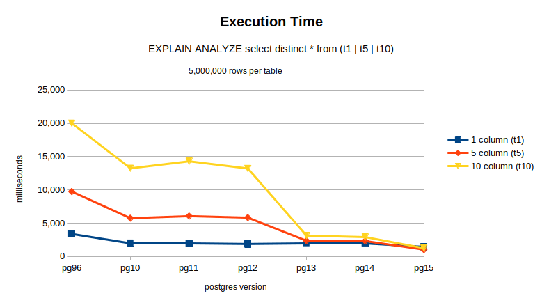
One of the more interesting aspects of the investigation was reviewing the query plans between different versions of Postgres. For example, the query plan for a single-column DISTINCT was quite similar between the Postgres 9.6 and Postgres 15 plans, ignoring the superior execution time.

                        PG96 QUERY PLAN, TABLE T1
-------------------------------------------------------------------------------
 Unique  (cost=765185.42..790185.42 rows=500 width=4) (actual time=2456.805..3381.230 rows=500 loops=1)
   ->  Sort  (cost=765185.42..777685.42 rows=5000000 width=4) (actual time=2456.804..3163.600 rows=5000000 loops=1)
         Sort Key: c1
         Sort Method: external merge  Disk: 68432kB
         ->  Seq Scan on t1  (cost=0.00..72124.00 rows=5000000 width=4) (actual time=0.055..291.523 rows=5000000 loops=1)
 Planning time: 0.161 ms
 Execution time: 3381.662 ms

PG96 QUERY PLAN, TABLE T1

-------------------------------------------------------------------------------

Unique (cost=765185.42..790185.42 rows=500 width=4) (actual time=2456.805..3381.230 rows=500 loops=1)

-> Sort (cost=765185.42..777685.42 rows=5000000 width=4) (actual time=2456.804..3163.600 rows=5000000 loops=1)

Sort Key: c1

Sort Method: external merge Disk: 68432kB

-> Seq Scan on t1 (cost=0.00..72124.00 rows=5000000 width=4) (actual time=0.055..291.523 rows=5000000 loops=1)

Planning time: 0.161 ms

Execution time: 3381.662 ms

                        PG15 QUERY PLAN, TABLE T1
---------------------------------------------------------------------------
 Unique  (cost=557992.61..582992.61 rows=500 width=4) (actual time=946.556..1411.421 rows=500 loops=1)
   ->  Sort  (cost=557992.61..570492.61 rows=5000000 width=4) (actual time=946.554..1223.289 rows=5000000 loops=1)
         Sort Key: c1
         Sort Method: external merge  Disk: 58720kB
         ->  Seq Scan on t1  (cost=0.00..72124.00 rows=5000000 width=4) (actual time=0.038..259.329 rows=5000000 loops=1)
 Planning Time: 0.229 ms
 JIT:
   Functions: 1
   Options: Inlining true, Optimization true, Expressions true, Deforming true
   Timing: Generation 0.150 ms, Inlining 31.332 ms, Optimization 6.746 ms, Emission 6.847 ms, Total 45.074 ms
 Execution Time: 1438.683 ms

PG15 QUERY PLAN, TABLE T1

---------------------------------------------------------------------------

Unique (cost=557992.61..582992.61 rows=500 width=4) (actual time=946.556..1411.421 rows=500 loops=1)

-> Sort (cost=557992.61..570492.61 rows=5000000 width=4) (actual time=946.554..1223.289 rows=5000000 loops=1)

Sort Key: c1

Sort Method: external merge Disk: 58720kB

-> Seq Scan on t1 (cost=0.00..72124.00 rows=5000000 width=4) (actual time=0.038..259.329 rows=5000000 loops=1)

Planning Time: 0.229 ms

JIT:

Functions: 1

Options: Inlining true, Optimization true, Expressions true, Deforming true

Timing: Generation 0.150 ms, Inlining 31.332 ms, Optimization 6.746 ms, Emission 6.847 ms, Total 45.074 ms

Execution Time: 1438.683 ms

The real difference appeared when the number of DISTINCT columns increased, as demonstrated by querying table t10. Here, parallelization is visible in the query plan.

                         PG96 QUERY PLAN, TABLE T10
-------------------------------------------------------------------------------------------
 Unique  (cost=1119650.30..1257425.30 rows=501000 width=73) (actual time=14257.801..20024.271 rows=50601 loops=1)
   ->  Sort  (cost=1119650.30..1132175.30 rows=5010000 width=73) (actual time=14257.800..19118.145 rows=5010000 loops=1)
         Sort Key: c1, c2, c3, c4, c5, c6, c7, c8, c9, c10
         Sort Method: external merge  Disk: 421232kB
         ->  Seq Scan on t10  (cost=0.00..116900.00 rows=5010000 width=73) (actual time=0.073..419.701 rows=5010000 loops=1)
 Planning time: 0.352 ms
 Execution time: 20025.956 ms

PG96 QUERY PLAN, TABLE T10

-------------------------------------------------------------------------------------------

Unique (cost=1119650.30..1257425.30 rows=501000 width=73) (actual time=14257.801..20024.271 rows=50601 loops=1)

-> Sort (cost=1119650.30..1132175.30 rows=5010000 width=73) (actual time=14257.800..19118.145 rows=5010000 loops=1)

Sort Key: c1, c2, c3, c4, c5, c6, c7, c8, c9, c10

Sort Method: external merge Disk: 421232kB

-> Seq Scan on t10 (cost=0.00..116900.00 rows=5010000 width=73) (actual time=0.073..419.701 rows=5010000 loops=1)

Planning time: 0.352 ms

Execution time: 20025.956 ms

                         PG15 QUERY PLAN, TABLE T10
-------------------------------------------------------------------------------------------
 HashAggregate  (cost=699692.77..730144.18 rows=501000 width=73) (actual time=1212.779..1232.667 rows=50601 loops=1)
   Group Key: c1, c2, c3, c4, c5, c6, c7, c8, c9, c10
   Planned Partitions: 16  Batches: 17  Memory Usage: 8373kB  Disk Usage: 2976kB
   ->  Gather  (cost=394624.22..552837.15 rows=1002000 width=73) (actual time=1071.280..1141.814 rows=151803 loops=1)
         Workers Planned: 2
         Workers Launched: 2
         ->  HashAggregate  (cost=393624.22..451637.15 rows=501000 width=73) (actual time=1064.261..1122.628 rows=50601 loops=3)
               Group Key: c1, c2, c3, c4, c5, c6, c7, c8, c9, c10
               Planned Partitions: 16  Batches: 17  Memory Usage: 8373kB  Disk Usage: 15176kB
               Worker 0:  Batches: 17  Memory Usage: 8373kB  Disk Usage: 18464kB
               Worker 1:  Batches: 17  Memory Usage: 8373kB  Disk Usage: 19464kB
               ->  Parallel Seq Scan on t10  (cost=0.00..87675.00 rows=2087500 width=73) (actual time=0.072..159.083 rows=1670000 loops=3)
 Planning Time: 0.286 ms
 JIT:
   Functions: 31
   Options: Inlining true, Optimization true, Expressions true, Deforming true
   Timing: Generation 3.510 ms, Inlining 123.698 ms, Optimization 200.805 ms, Emission 149.608 ms, Total 477.621 ms
 Execution Time: 1244.556 ms

PG15 QUERY PLAN, TABLE T10

-------------------------------------------------------------------------------------------

HashAggregate (cost=699692.77..730144.18 rows=501000 width=73) (actual time=1212.779..1232.667 rows=50601 loops=1)

Group Key: c1, c2, c3, c4, c5, c6, c7, c8, c9, c10

Planned Partitions: 16 Batches: 17 Memory Usage: 8373kB Disk Usage: 2976kB

-> Gather (cost=394624.22..552837.15 rows=1002000 width=73) (actual time=1071.280..1141.814 rows=151803 loops=1)

Workers Planned: 2

Workers Launched: 2

-> HashAggregate (cost=393624.22..451637.15 rows=501000 width=73) (actual time=1064.261..1122.628 rows=50601 loops=3)

Group Key: c1, c2, c3, c4, c5, c6, c7, c8, c9, c10

Planned Partitions: 16 Batches: 17 Memory Usage: 8373kB Disk Usage: 15176kB

Worker 0: Batches: 17 Memory Usage: 8373kB Disk Usage: 18464kB

Worker 1: Batches: 17 Memory Usage: 8373kB Disk Usage: 19464kB

-> Parallel Seq Scan on t10 (cost=0.00..87675.00 rows=2087500 width=73) (actual time=0.072..159.083 rows=1670000 loops=3)

Planning Time: 0.286 ms

JIT:

Functions: 31

Options: Inlining true, Optimization true, Expressions true, Deforming true

Timing: Generation 3.510 ms, Inlining 123.698 ms, Optimization 200.805 ms, Emission 149.608 ms, Total 477.621 ms

Execution Time: 1244.556 ms

Increasing Performance

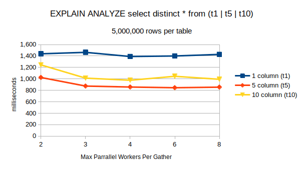
Performance enhancements were made by updating the Postgres runtime parameter max_parallel_workers_per_gather. The default value in a newly initialized cluster is 2. As the table below indicates, performance quickly reached diminishing returns due to the restricted capabilities of the testing hardware.

POSTGRES VERSION 15

max_parallel_workers_per_gather	1 column (t1)	5 column (t5)	10 column (t10)
2	1,439	1,025	1,245
3	1,464	875	1,013
4	1,391	858	977
6	1,401	846	1,045
8	1,428	856	993

PostgreSQL Distinct

About Indexes

Performance improvements were not realized when indexes were applied as demonstrated in this query plan.

PG15, table t10 with 10 DISTINCT columns and max_parallel_workers_per_gather=4:

                                     QUERY PLAN
-----------------------------------------------------------------------------------
 Unique  (cost=0.43..251344.40 rows=501000 width=73) (actual time=0.060..1240.729 rows=50601 loops=1)
   ->  Index Only Scan using t10_c1_c2_c3_c4_c5_c6_c7_c8_c9_c10_idx on t10  (cost=0.43..126094.40 rows=5010000 width=73) (actual time=0.058..710.780 rows=5010000 loops=1)
         Heap Fetches: 582675
 Planning Time: 0.596 ms
 JIT:
   Functions: 1
   Options: Inlining false, Optimization false, Expressions true, Deforming true
   Timing: Generation 0.262 ms, Inlining 0.000 ms, Optimization 0.122 ms, Emission 2.295 ms, Total 2.679 ms
 Execution Time: 1249.391 ms

QUERY PLAN

-----------------------------------------------------------------------------------

Unique (cost=0.43..251344.40 rows=501000 width=73) (actual time=0.060..1240.729 rows=50601 loops=1)

-> Index Only Scan using t10_c1_c2_c3_c4_c5_c6_c7_c8_c9_c10_idx on t10 (cost=0.43..126094.40 rows=5010000 width=73) (actual time=0.058..710.780 rows=5010000 loops=1)

Heap Fetches: 582675

Planning Time: 0.596 ms

JIT:

Functions: 1

Options: Inlining false, Optimization false, Expressions true, Deforming true

Timing: Generation 0.262 ms, Inlining 0.000 ms, Optimization 0.122 ms, Emission 2.295 ms, Total 2.679 ms

Execution Time: 1249.391 ms

Concluding Thoughts

Running DISTINCT across multiple CPUs is a significant performance improvement. However, keep in mind the risk of diminishing returns as you increase max_parallel_workers_per_gather and approach your hardware’s limitations. As the investigation showed, under normal circumstances, the query planner may decide to use indexes instead of running parallel workers. One way to work around this is to consider disabling runtime parameters such as enable_indexonlyscan and enable_indexscan. Finally, run EXPLAIN ANALYZE to understand what is happening.

Get Percona Support for PostgreSQL

Percona supports DBAs and developers seeking help with their PostgreSQL databases.

Percona Support for PostgreSQL

Additional Percona support and resources include:

Percona Distribution for PostgreSQL Software

Percona Platform

Percona Managed Services

Percona Professional Services

0 0 votes

Article Rating

6 Comments

Oldest

Newest Most Voted

Inline Feedbacks

View all comments

Oliver

3 years ago

Good to see, thank you.

I see that the query is spilling to disk – from the query plan:

Sort Method: external merge Disk: 68432kB

It would be interesting to see the timing results if the machine is configured with enough memory and/or suitable work_mem etc. parameters so that that doesn’t happen, which would give a more representative use. Otherwise the disk activity could swamp pretty much every other factor.

Author

rbernier01

3 years ago

Reply to Oliver

Hi, It’s an excellent point!

I’m always 2nd guessing myself how much tuning I should perform whenever I do one of these investigations. Over time I’ve realized that so long as the methodology and assumptions are documented then there’s hopefully enough information presented that it can be used at least as a starting point satisfying the reader’s own needs.

Hope this helps 🙂

Author

rbernier01

3 years ago

It’s a good point. I think that so long as there’s enough information allowing its replication then people can hopefully takie what they’ve read as a starting point for their own investigations.

Peter Gram

3 years ago

you write “This SQL statement returns those records filtering out the UNIQUE values found in column “c1” in SORTED order: select distinct on(c1) * from t_ex;”.
The SQL standard is open to if distinct should return data sorted or random since this i implementation dependent. Oracle used to return values from “distinct” and “group by” sorted but from version 9.x this is not true longer since they started to use a hash parallel function and after this values are not sorted.
The official statement is if you need data in sorted order use a “order by”.

Fazal Majid

3 years ago

It’s worth mentioning that at scale no one uses SELECT DISTINCT but instead fast approximate methods like HyperLogLog as implemented in CitusData’s postgresql-hll:

https://github.com/citusdata/postgresql-hll