
Based on my Percona Live 2026 talk “On-disk and Redis Compatible: Evaluating Kvrocks.” I will cover benchmarking Kvrocks in a separate post.
We all run Valkey or Redis for well-known reasons: all the data lives in RAM, and it’s fast. Storing data in RAM is of course expensive. Once your dataset grows into the tens or hundreds of terabytes, the question stops being “how fast is it?” and becomes “how many servers, and how much memory?” Or more specifically “how much is this going to cost?”.
Apache Kvrocks provides an interesting answer to that question. It stores data on disk using RocksDB instead of holding it in memory, and it speaks the RESP protocol, so that your existing Redis and Valkey clients work against it. Kvrocks is an Apache Software Foundation (ASF) project (Apache 2.0 licence), open source since 2019, and is widely deployed in production, particularly in Asia by internet-scale organisations like Baidu and Trip.com (Apache Kvrocks users list).
Throughout this post, I’m using Valkey as a comparison. Everything said about Valkey applies to Redis.
Intuitively, you’d expect Kvrocks’ latency to sit somewhere between an in-memory store like Valkey and a disk-based relational database. That’s roughly right, but exactly where depends almost entirely on your workload. Understanding why the workload matters so much becomes clear from how it stores data and that’s what this post is about.
The simplest mental model: a Kvrocks node is a thin layer on top of RocksDB (rocksdb-101). The graphic below shows the main components of a Kvrocks node.
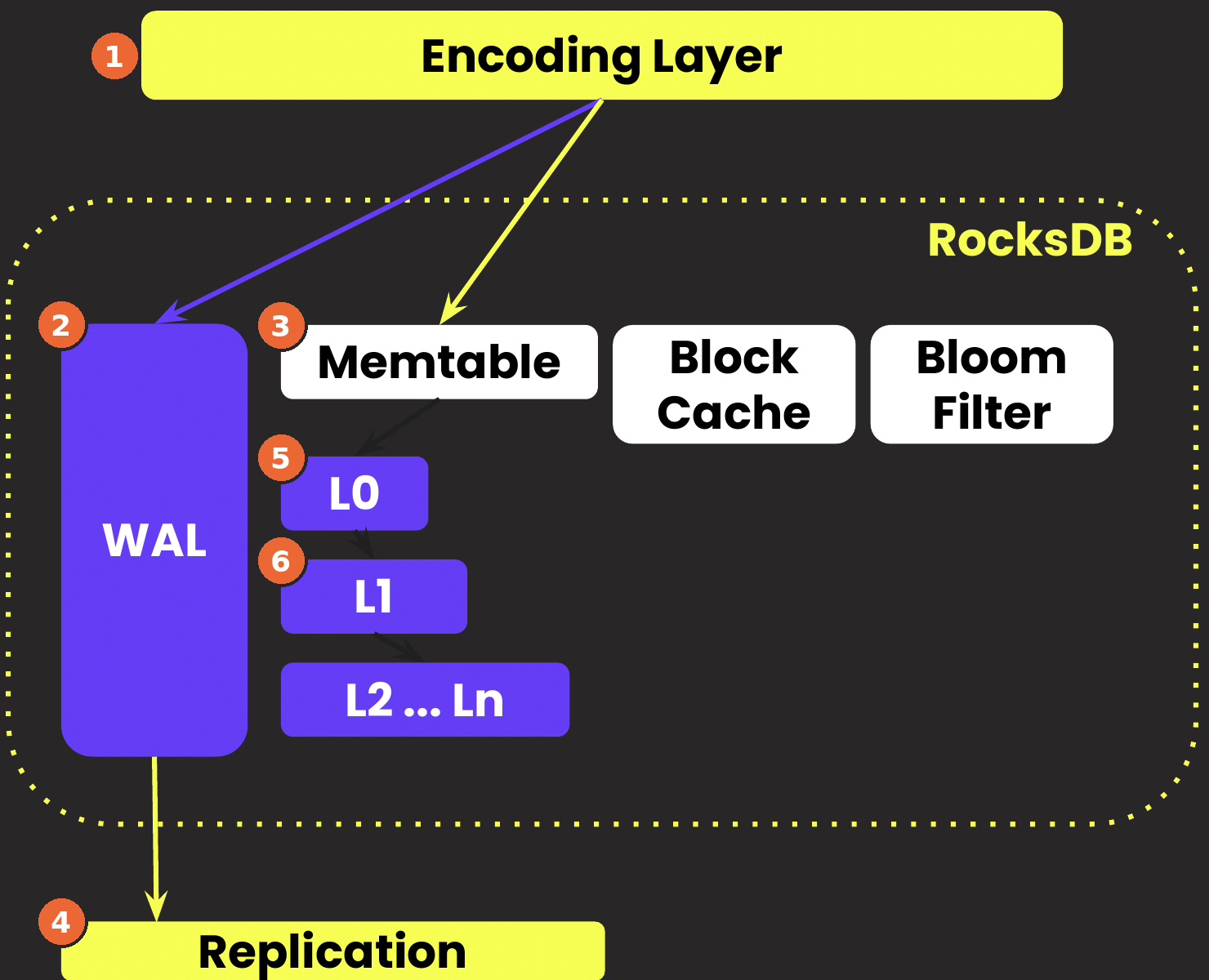
The numbers in the diagram show the order of a write.
In the same diagram, the RocksDB components block cache and bloom filters live in memory just like memtables. The block cache holds recently read blocks from the SST files; the bloom filters help to skip files for a read that definitely don’t contain the key it’s looking for.
By default the WAL is written but not synced on each write. So similar to Valkey’s appendfsync no which means that a write survives a Kvrocks crash, but not a power failure. Setting rocksdb.write_options.sync yes gives you the equivalent of appendfsync always.
If you’ve worked with MyRocks or any other RocksDB-based system, most of this will look familiar. What’s specific to Kvrocks is how Valkey data types are mapped onto RocksDB keys.
RocksDB only knows about ordered byte-string keys and values. Valkey has strings, hashes, lists, sets, sorted sets and more. The encoding has two patterns.
Strings are the simple case: the value is stored inline with the key. There are no subkeys.
Collections (hashes, lists, sets, sorted sets) get one metadata entry for the key, plus one versioned subkey row per element. Here’s what a small hash looks like:
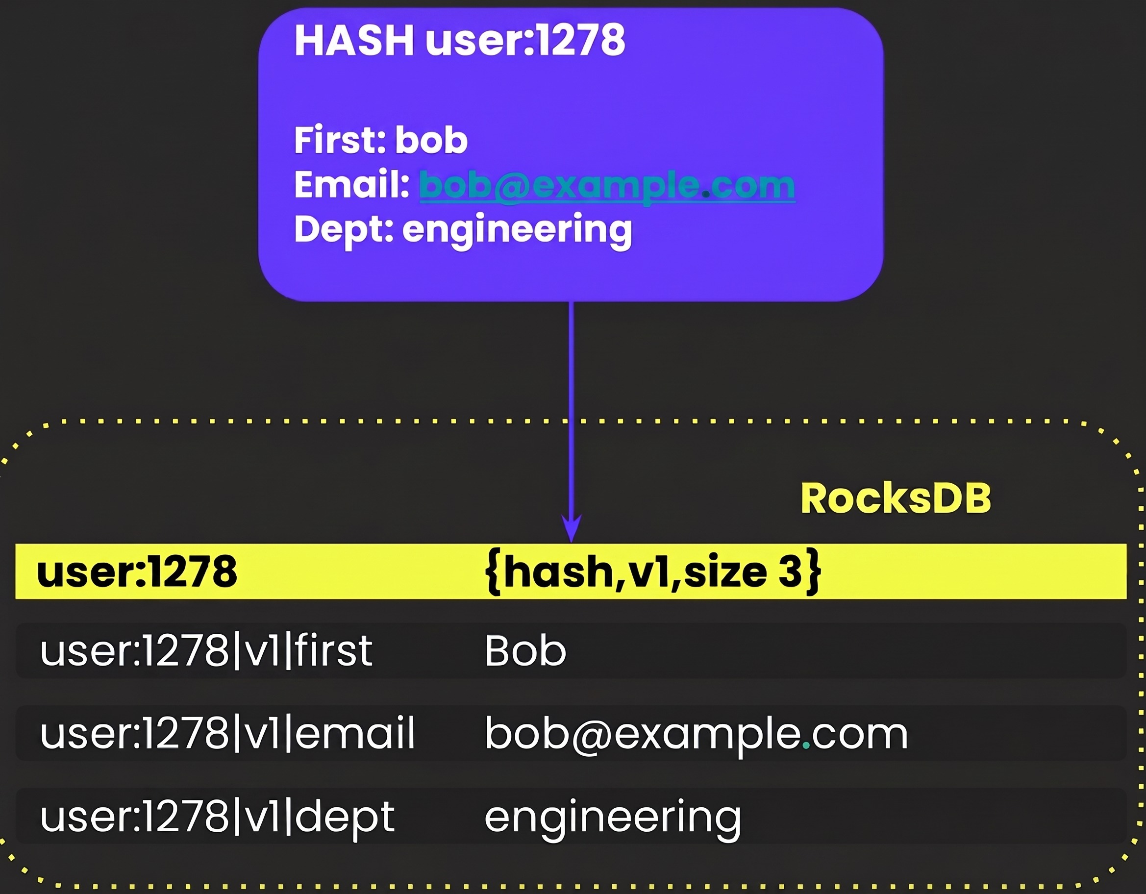
The metadata entry for user:1278 records the type (hash), a version and the size (3 fields). The version is shown as v1 for readability. In practice it’s a 64-bit generated value at creation time. If the key has a TTL, that also lives in the metadata. Each field then becomes its own RocksDB row, keyed by the user key, the version and the field name: user:1278|v1|first, user:1278|v1|email, and so on. The real encoding also prefixes every key with a namespace and the slot ID in cluster mode. It is also length-prefixed rather than using separators. The simplified form shows this structure.
A single HASH therefore ends up as multiple keys in RocksDB. To guarantee atomicity, multi-key changes are processed as a rocksdb::WriteBatch. RocksDB applies that as an all-or-nothing operation.
Other Valkey types follow the same pattern with small variations. Lists store head and tail indices in their metadata, so pushes and pops at either end are cheap. Sorted sets get an additional score index so that range-by-score queries become an ordered seek rather than a scan.
The version number in every subkey comes in very handy for deletes. An LSM tree doesn’t update data in place the way InnoDB or PostgreSQL update data pages; it appends. So how do you delete a hash with a million fields without writing a million tombstones?
You don’t. A delete only removes the metadata entry, which is a single write. The subkey rows are left where they are. Every read of an element starts from the metadata, so with the metadata gone the whole collection is gone as far as clients are concerned.
The version is what keeps those leftover rows harmless. If user:1278 is created again, it gets a new metadata entry with a new version, and its fields are written as user:1278|v2|... The old user:1278|v1|... rows can never match the live metadata. They are orphaned and inaccessible.
The space isn’t reclaimed immediately. That happens during SST file compaction. Kvrocks installs a compaction filter that checks each subkey row it encounters against the current metadata for its key, and drops the row if the metadata is missing, carries a different version, or has expired. Expiry works the same way. Once a key’s TTL has passed, reads treat it as absent, and compaction later removes both its metadata and its subkeys.
Valkey handles deletes in a different way. A DEL (or UNLINK) on a large collection removes the key from the keyspace immediately and hands the memory to a background thread to free. Valkey has done this since lazyfree-lazy-user-del became default yes. Deletes are O(1) for the client in both Valkey and Kvrocks. With Valkey the memory comes back almost at once and with Kvrocks the disk space comes back when compaction deals with it. Frequently deleting and recreating large collections thus shows as extra disk usage until the deleted data has been cleaned up.
Kvrocks separates its data into RocksDB column families (CFs), each with its own memtables and SST files:
default in RocksDB) holds one entry per collection element.zset_score) holds the score index for sorted sets.stream) holds stream entries.search) holds secondary index data for the FT.* search commands, including vector (HNSW) indexes.index) holds the label index for time series.pubsub) carries published messages through the WAL so they reach replicas.propagate) stores Lua scripts, functions and namespace tokens, and carries commands to replicas that aren’t data writes.One important difference from Valkey: there is no in-memory dictionary of keys. In Valkey, every key lives in a hash table in RAM. In Kvrocks, the keyspace is the LSM tree. Two billion keys don’t need two billion entries in memory. They need metadata rows on disk, plus whatever portion of them you choose to keep cached.
How a write flows through the system.
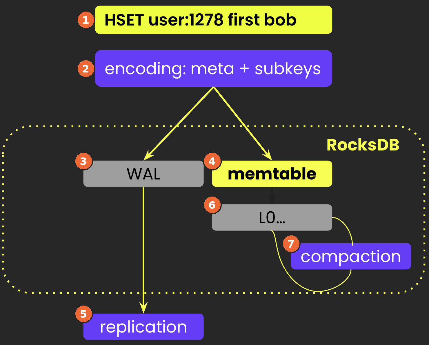
HSET user:1278 first bob arrivesThis means that a given row may be rewritten several times over its lifetime as it moves down through the levels. Called write amplification, this is a function of the LSM tree turning random writes into sequential ones. For large values under a heavy write load this is the biggest source of latency trouble.
Reads work their way from the fastest storage to the slowest.
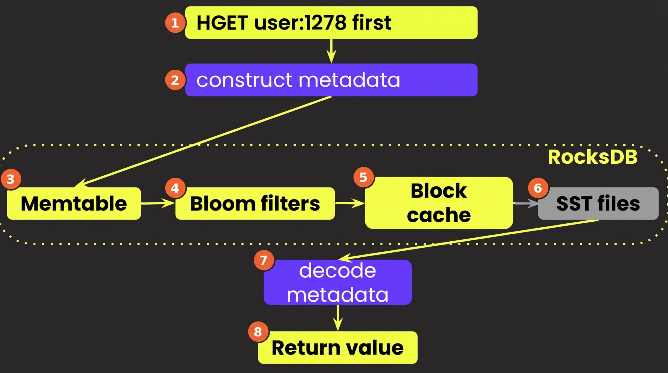
HGET user:1278 first arrivesuser:1278 to learn its type, its current version and whether it has expired. The subkey is then built using user:1278|v1|first.Each lookup follows the same order. First the memtables are checked and if the row was written recently, it’s found in memory. If not, RocksDB works through the SST files, newest level first. For each candidate SST file, the bloom filter for that SST file is checked before anything is read. The bloom filter will rule out files it cannot be in. For a file that might hold the key, RocksDB needs the relevant index and data blocks. These can be in the block cache or have to be read from file.
The important line is the one between “block cache hit” and “block cache miss.” A hit costs you a memory lookup. A miss goes to the filesystem, and unless the block is in the operating system’s page cache it becomes a disk read. Kvrocks performance can be summarised as how often you cross that line, and how fast storage is when you do. With the Kvrocks caches and the OS page cache, RAM still matters even if it’s an “on-disk” database.
Everything above describes a point lookup like HGET. Commands that return a range like HGETALL work differently. Because every subkey row of a collection starts with the same user key|version, RocksDB’s key ordering stores all of a collection’s elements next to each other. A range read jumps to the first element, user:1278|v1|..., and reads forward row by row until it reaches the end of that collection. Bloom filters can’t help with that, because they only answer whether an exact key might be in a file. Kvrocks also deliberately doesn’t add blocks read by a scan to the block cache, so one large HGETALL can’t evict your hot data. The downside is that repeated scans of the same large collection depend on the OS page cache, not on Kvrocks’ own caches. Multi-field point reads like HMGET are batched point lookups and behave like HGET.
So two workloads with the same dataset size can perform very differently, depending on whether they read single elements or whole collections.
Kvrocks scales out using the same model as Valkey Cluster: 16384 hash slots divided among primaries, each with its own replicas. Standard cluster-aware clients work as-is.
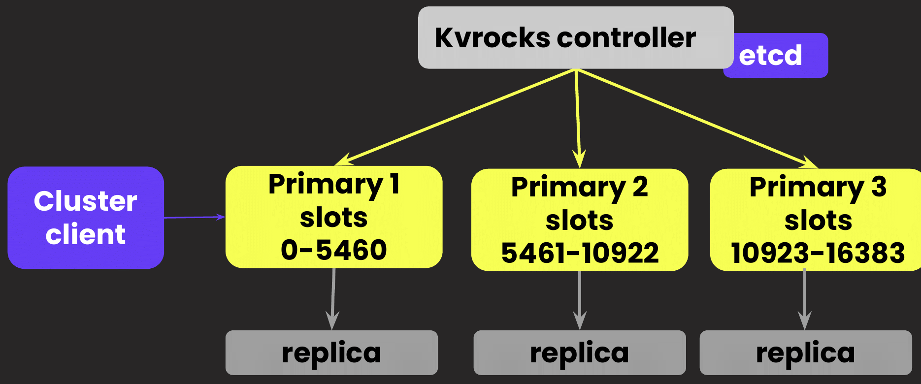
The big difference is how the topology is managed. In Valkey Cluster, every node gossips with every other node, and on a large cluster that becomes a lot of chatter. Kvrocks does not use the gossip protocol. Nodes don’t discover each other but instead the topology is pushed to the nodes via the CLUSTERX SETNODES command. This is the job of the Kvrocks controller which is the owner of the topology. It handles failover and keeps its state in an external store such as etcd.
Scaling out works the way you would expect for a Valkey-style cluster. Add a shard and then migrate slots to it. During migration the data for a slot is copied to the new shard while writes keep arriving. At the end there’s a brief pause while the final changes are caught up and ownership switches over. It is short, but it’s important to keep in mind when you have tight tail-latency requirements during rebalancing.
Multi-key operations need all their keys in the same slot, so use hash tags exactly as with Valkey Cluster. A difference with Valkey is that the on-disk data format in cluster mode includes the slot ID. That means a standalone node’s data isn’t in cluster format. Moving from standalone to cluster mode thus becomes a data migration.
Every read that misses the in-memory caches becomes a disk read. So performance doesn’t depend directly on how big your dataset is. It depends on how often your workload misses the cache, how fast your storage is, and whether your storage can keep up with those misses.
Every write gets rewritten as the compaction process moves it down the LSM tree. So your write rate determines how much background work competes with your foreground application traffic.
Those two facts make up every trade-off in running Kvrocks. In the next blog, I’ll put some numbers on performance by walking through a real 500 TB use case, and provide a checklist for deciding whether your workload belongs on Kvrocks, Valkey or another database.
Based on customer demand, Percona now supports Kvrocks alongside Valkey and Redis. To find out more about Kvrocks:
Resources
RELATED POSTS