

Nearly every database has vector search now, and every one of them has a blog post with a big number in it. Almost none of those numbers can be checked, because the thing that makes them meaningful is usually missing.
We built a vector-bench to stop guessing. You name the engines you want, build them from pinned versions, put each one in the same container on the same cores with the same data, run the same measurements against all of them, and write a report. This post is about how it measures.
If you work with databases but haven’t touched vectors yet, the first half is the part you need.
What’s being indexed
An embedding is a fixed-length array of floats that comes out of a model. The useful property is that semantically similar inputs land close together when you measure the distance between them.
Two distance measures cover almost everything. L2 is an ordinary straight-line distance, the Pythagorean one, extended to however many dimensions you have. Cosine Similarity measures the angle between two vectors and ignores their length. Which one applies is decided by the model that produced the embeddings. It isn’t a choice you get to make at query time, and getting it wrong is a good way to produce nonsense.
So the query you want is “the 10 rows whose vectors are nearest this one”:
|
1 |
SELECT id FROM documents ORDER BY distance(embedding, ?) LIMIT 10; |
That 10 is k.
Now the problem. Answering that exactly means computing the distance from your query vector to every single row, then sorting. No B-tree or hash index helps, because neither one can order a million points by proximity in 1536 dimensions. Exact vector search is a full table scan with a lot of arithmetic bolted on.
A vector index gives up exactness to avoid that. It looks at a few thousand promising candidates instead of every row and returns the best it found. That’s the approximate nearest neighbour search, or ANN. It’s usually right.
“Usually” is doing a lot of work in that sentence, and pinning it down is most of what this benchmark does.
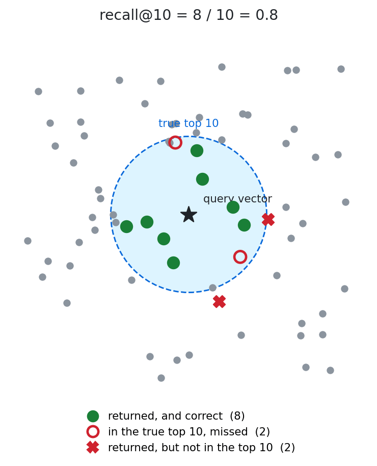
To score that you need to know the right answer in the first place. That’s the ground truth: the true nearest neighbours for every query, computed once by brute force with no index involved. The public ANN datasets ship theirs alongside the vectors, and without it you couldn’t score an approximate index at all.
This is the number that makes everything else meaningful, and it’s the one most vector search claims leave out. That omission is the reason this project exists.
Almost every database that has added vector search picked one of two designs. They attack the same problem from opposite ends, and which one you have decides what you’re allowed to tune.
HNSW stands for Hierarchical Navigable Small World, which is a mouthful for something fairly intuitive. If you’ve ever implemented a skip list, you already have the shape of it.
It’s a graph of vectors built in layers. Every vector is a node, linked to some number of its nearest neighbours. The top layer has few nodes and its links jump long distances across the data. Each layer below has more nodes and shorter links. A search starts at the top and keeps hopping to whichever neighbour is closer to the query. When nothing is closer, it drops a layer and carries on, until it runs out of layers.
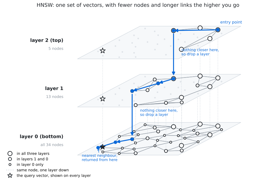
Two settings matter:
There’s ef_construction too, the same idea applied while the index is being built. Not every engine lets you set it, which turns out to matter when you try to compare them fairly.
IVF stands for Inverted File. It partitions the data instead of linking it, not unlike list partitioning on a table.
At build time it groups the vectors into nlist clusters, each with a representative vector at its centre. At query time it compares the query against those representatives, picks the closest nprobe clusters, and searches only inside them. It builds much faster than HNSW and uses less memory, but usually gives worse recall at the same speed. It misses when the true neighbour happens to sit just outside the clusters it looked in.
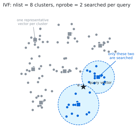
We only test engines running HNSW, which is what most databases shipped. Putting an IVF engine on the same chart would mostly measure the gap between two algorithms rather than how well anybody implemented one, so IVF-only engines get their own bucket.
Recall isn’t a property of an engine. It’s a setting, and ef_search is the dial.
Here’s one HNSW index on one machine, same data, same queries. The only difference is that on the first row the search tracks 10 candidate nodes as it walks the graph, and on the second it tracks 800:
|
1 2 |
ef_search=10 3,678 queries/sec recall 0.9593 ef_search=800 409 queries/sec recall 0.9987 |
Keeping 800 candidates instead of 10 finds a better answer and takes nine times as long. Both rows are honest measurements of the same index on the same hardware.
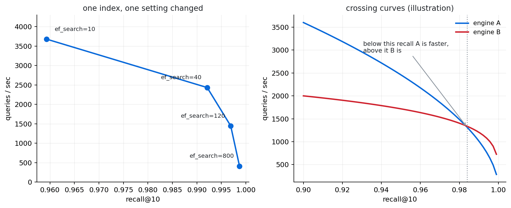
Which is why “our database does 3,678 vector queries a second” tells you nothing. You don’t know how often it was handing back the wrong rows, and the person quoting it may not know either. The reverse is just as empty: recall with no throughput next to it is free, because recall 1.0 is always available if you turn the index off and scan the table.
Every measurement here is a pair. If you take one thing from this post, take that.
One table per engine. An id, an integer tag column used only by the filtered tests, the vector, and an HNSW index on it at a configured M.
|
1 2 3 4 5 |
CREATE TABLE t1 ( id INTEGER PRIMARY KEY, tag INTEGER NOT NULL, v VECTOR(1536) ); |
Then two queries, plain top-k and the same search restricted to a subset of rows:
|
1 2 |
SELECT id FROM t1 ORDER BY distance(v, ?) LIMIT 10; SELECT id FROM t1 WHERE tag < ? ORDER BY distance(v, ?) LIMIT 10; |
tag holds values 0 to 99 spread evenly, so tag < 10 passes about 10% of rows and tag < 1 about 1%. That’s how we control selectivity.
Every engine writes all of this differently. Some declare the index inside CREATE TABLE, others want a separate CREATE INDEX, and the distance functions have different names everywhere. Translating that is the driver’s job, and the drivers are the only engine-specific code in the whole harness.
Every engine also has at least one setup detail that will quietly wreck your numbers. PostgreSQL, for instance, stores oversized values out of line in what it calls TOAST, and a 1536-dimension vector counts as oversized. Unless the column is set to STORAGE PLAIN, every single distance comparison pays for an extra fetch. It’s one line of DDL. Miss it and you publish PostgreSQL looking slow for a reason that has nothing to do with its vector search, and you’d never know from the results.
Recall against throughput. Iterate ef_search against a fixed index, record recall and QPS at each point, repeat at a few values of M. k=10 throughout. The query vectors come from the dataset’s own held-out query set, never from the rows we loaded, because searching for a vector that’s already in the index is a much easier problem and would flatter everybody equally.
The two settings behave completely differently, and it shapes how long a run takes. ef_search is a session variable, so iterating it reuses the index that’s already built and each extra point costs almost nothing. M is baked into the index, so every value of M means dropping the table and loading the entire dataset again. On a million 1536-dimension vectors that’s hours per value. Hence many ef_search points and very few M values.
Build cost. Wall time, rows per second, index size on disk, peak memory.
This is the easiest place in the whole benchmark to publish a misleading number, because engines don’t build the index the same way. Engines can build indexes either incrementally, bulk, or both. What does that mean?
Incremental. The graph is updated on every INSERT. Loading is slow, but when the last row lands the index is finished and the table is ready to query.
Bulk. All the rows load first, then the whole graph gets built in one pass. Much faster in total, but the table can’t answer a vector query until the build finishes.
Those are two different operations. One engine in our set does both, and its bulk path loaded 18 times more rows per second than its own incremental path. Same engine, same data, same machine, 18x apart.
So a bulk number from one engine put next to an incremental number from another doesn’t compare engines at all. It compares two ways of building an index, and the ratio looks impressive enough that people quote it anyway. We measure both paths on any engine that has both, and the report says which is which.
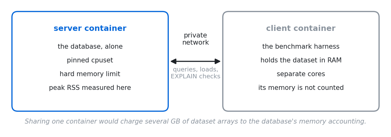
Peak memory comes from the server’s container, with the database as the only thing running in it. The harness runs in a separate container and reaches the server over a private network.
That separation matters more than it sounds. The client holds the entire dataset in memory, several GB of Python arrays. If it shared a container with the database, the container’s memory accounting would count those arrays as database memory, and every memory figure we published would be inflated by whatever the client happened to be holding.
Concurrency. QPS and latency percentiles from 1 to 32 clients. Engines cache their graphs in quite different ways and none of that shows up until clients start competing for the same cache. We report how much of the ideal speedup each engine actually got alongside raw QPS, because an engine that stops gaining throughput at 2 clients while its p99 gets 15 times worse is doing something very different from one that keeps scaling, and a throughput column on its own hides that completely.
Filtered search, at several selectivities down to 1% of rows passing. This is the case that’s supposed to justify keeping vectors in your database instead of a dedicated store, so it deserves more attention than it usually gets.
Filtering changes what “correct” means. The true top 10 among rows where tag < 10 is not the true top 10 overall, so for every selectivity we recompute ground truth by brute force over only the rows that pass. Score filtered results against the unfiltered ground truth that shipped with the dataset and every engine gets a recall near zero. We know, because we did exactly that for a while.
Some queries come back with fewer than 10 rows. In one run, 81 out of 200 did. This is not the data running out. At 10% selectivity about 99,000 rows pass the filter, so there are always at least 10 to find. The cause is the order of the operations. HNSW searches by distance first, then applies the WHERE clause. It gathers a few thousand candidates, the filter throws most of them away, and sometimes fewer than 10 are left. (If a filter really did match fewer than 10 rows, the ground truth shrinks too, and the engine still scores 1.0.) Recall already handles this. A row the engine did not return counts as a miss, so six correct rows score 0.6. We report the count because two different problems score the same. “10 rows, four of them wrong” and “six rows, all correct” are both 0.6. The first needs a wider search. The second needs iterative scanning. The count tells you which one you have. It also means the throughput is flattered, since six rows is less work than ten.
Churn. Recall and throughput before and after deleting and reinserting part of the corpus, since deletions leave graph edges pointing at rows that are gone. Whether rebuilding the index recovers what’s lost, we don’t know yet. It’s the obvious next thing to test and we haven’t done it.
Everything runs twice.
The normalized pass gives every engine identical CPU, memory and cache budgets, so a difference in the results belongs to the implementation rather than to who was handed more RAM. The tuned pass lets each engine use the settings its own documentation recommends. Tuned is more realistic and less controlled, which is exactly why it doesn’t replace the first one. A result that survives both passes is about the engine. One that flips between them is interesting for a completely different reason.
Cores are pinned explicitly. One logical CPU per physical core, because SMT siblings share execution units and two threads on one core don’t behave like two cores. Never a mix of P-cores and E-cores on hybrid chips either, since migration between core types adds more variance than several of the effects we’re trying to measure. Durability is relaxed the same way everywhere, or we’d be comparing default fsync policies and calling it vector search.
Some differences can’t be equalised at all, so we write them down instead of pretending. A knob only one engine exposes goes unused in the normalized pass, because using it would hand that engine a tuning axis nobody else has. An engine that insists on a particular isolation level gets it set for everyone. And defaults that are obviously placeholders get sized from a shared budget — one family of engines still ships a 16 MiB graph cache, which is nothing, and judging an engine on a value its own vendor expects you to change measures absolutely nothing. All of these land in a “known asymmetries” section above the results.
One hardware note that catches people out. Several of these implementations ship hand-written AVX-512 code for the distance maths, where a single instruction does the arithmetic for 16 floats at once. The same index on a CPU without AVX-512 is effectively a different benchmark, and the slowdown isn’t the same for every engine, so you can’t even scale the numbers to compensate. The CPU model and its feature flags go into every run’s manifest for that reason, along with engine versions and commits, image IDs, and the resource limits as they are actually resolved rather than as we requested them. No manifest, no report.
Read the validity section before you look at a single chart. Our reports go environment, then validity, then known asymmetries, then results, in that order on purpose. A failed phase, an engine returning short result sets, a CPU missing the instruction set the engines wanted — all of it lands in front of you before you’ve formed an opinion.
The thing to watch for is the silent full scan.
Any of these engines will quietly stop using the vector index and scan the table instead. A scan returns exact results, slowly, so in the output it looks like high recall and low throughput. That’s indistinguishable from a conservatively tuned index unless you go and read the query plan.
It happens for thoroughly boring reasons. One engine’s optimizer costs the vector index against a table scan and takes the scan once the LIMIT is above roughly a quarter of the table, and we still haven’t found a setting that moves it. Another falls back with no error and no warning when the query asks for a different distance than the index was built for — build the index for cosine, write the query with the L2 operator, and you get a sequential scan and a sort, with nothing anywhere to tell you.
So every driver runs EXPLAIN for each configuration and checks the index name appears in the plan.
WARNING: vector index NOT used (k=10, filtered=True). Plan: …Seq Scan…
Anything that is scanned goes into validity. This is far and away the easiest way to produce impressive vector benchmark numbers by accident, and if a benchmark doesn’t mention checking for it, we’d want to know why before believing anything in it.
For recall against throughput, the useful presentation is a curve rather than a number. Iterate ef_search, plot recall against QPS, keep the best points: for each level of accuracy, the highest throughput anything reached at it. One engine beats another only where its curve sits above the other’s at the same recall. If the curves cross, then the answer genuinely depends on how accurate you need to be, and saying so is a result rather than a dodge.
Curves do invite comparing shapes instead of heights at one point, so there are bar charts as well, QPS at recall floors of 0.90, 0.95 and 0.99. Pick the accuracy you’d actually accept and read across.
Worth listing, partly because they’re the reason to trust anything else here, and partly because anyone building something similar will walk into them.
Our first ingest numbers were garbage. The load path was doing one INSERT per network round trip with autocommit on, and we measured 88 rows a second. Batching 500 rows per transaction took the same engine to 373. Publishing the first number would have been benchmarking our own client and calling it a database.
Filtered search and churn were scored against full-corpus ground truth even on runs that used a subset of rows. Every engine looked bad and the bug was entirely ours. Ground truth is now keyed on dataset, k, row count and selectivity.
Both resource passes shared one results directory, and the ANN runner skips configurations that already have results. So the tuned pass quietly skipped everything the normalized pass had computed, and our tuned numbers were mostly normalized numbers wearing a different label. That one took an embarrassingly long time to notice.
Readiness probes lie. One engine’s standard “are you accepting connections” check returns success before the database it’s supposed to create actually exists. The probe passed, the first query failed, and we spent a while convinced it was an engine problem.
The most recent one, on a 1536-dimension corpus. The ANN runner holds the whole dataset in memory twice, once in the parent process and again in a forked worker, and the copies aren’t shared. That’s roughly 12 GB for a million embeddings, on top of whatever the server is using, in a container we’d sized for the server alone. The kernel killed the worker. The runner doesn’t check worker exit codes, so it logged “Terminating 1 workers”, exited successfully and wrote no results — which looks exactly like a run that had nothing left to do. Three hours to fail, and it failed silently.
This is the part we cared most about getting right, because the whole point was to avoid rebuilding the apparatus every time somebody ships vector search. Each engine needs:
Results, published with the manifests and the raw per-configuration records, so you can check them instead of taking our word for it.
Everything is at https://github.com/Percona-Lab/vector-bench harness, drivers, Dockerfiles, docs. If we’re measuring something wrong, or being unfair to an engine you know better than we do, tell us.
Resources
RELATED POSTS