Downloads

Blog

Shard-Query turbo charges Infobright community edition (ICE)

May 6, 2011

Author

Justin Swanhart

MySQL

Share this Post:

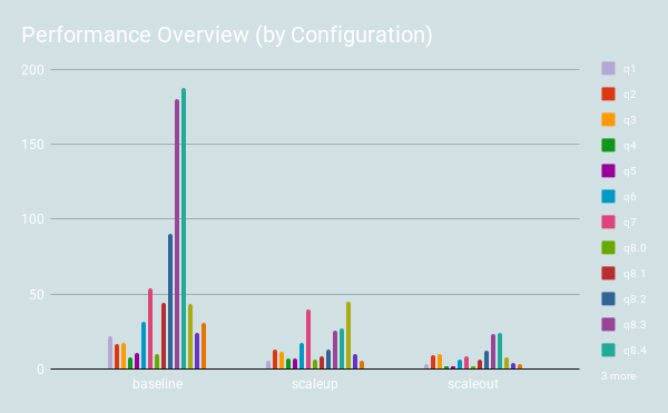
Shard-Query is an open source tool kit which helps improve the performance of queries against a MySQL database by distributing the work over multiple machines and/or multiple cores. This is similar to the divide and conquer approach that Hive takes in combination with Hadoop. Shard-Query applies a clever approach to parallelism which allows it to significantly improve the performance of queries by spreading the work over all available compute resources. In this test, Shard-Query averages a nearly 6x (max over 10x) improvement over the baseline, as shown in the following graph:

One significant advantage of Shard-Query over Hive is that it works with existing MySQL data sets and queries. Another advantage is that it works with all MySQL storage engines.

This set of benchmarks evaluates how well Infobright community edition (ICE) performs in combination with Shard-Query.

Data set

It was important to choose a data set that was large enough to create queries that would run for a decent amount of time, but not so large that it was difficult to work with. The ontime flight performance statistics data, available online from the United States Bureau of Transportation Statistics (BTS) made a good candidate for testing, as it had been tested before:
Another MPB post
Lucid DB testing

The raw data is a completely denormalized schema (single table). In order to demonstrate the power of Shard-Query it is important to test complex queries involving joins and aggregation. A star schema is the most common OLAP/DW data model, since it typically represents a data mart. See also: “Data mart or data warehouse?”. As it is the most common data model, it is desirable to benchmark using a star schema, even though it involves work to transform the data.

Star schema

Transforming the data was straightforward. I should note that I did this preprocessing with the MyISAM storage engine, then I dumped the data to tab delimited flat files using mysqldump. I started by loading the raw data from the BTS into a single database table called ontime_stage.

Then, the airport information was extracted:

create table dim_airport(<br>airport_id int auto_increment primary key,<br>unique key(airport_code)<br>)<br>as<br>select<br>  Origin as `airport_code`,<br>  OriginCityName as `CityName`,<br>  OriginState as `State`,<br>  OriginStateFips as `StateFips`,<br>  OriginStateName as `StateName` ,<br>  OriginWac as `Wac`<br>FROM ontime_stage<br>UNION<br>select<br>  Dest as `airport_code`,<br>  DestCityName as `CityName`,<br>  DestState as `State`,<br>  DestStateFips as `StateFips`,<br>  DestStateName as `StateName` ,<br>  DestWac as `Wac`<br>FROM ontime_stage;<br>

create table dim_airport( airport_id int auto_increment primary key, unique key(airport_code) ) as select Origin as `airport_code`, OriginCityName as `CityName`, OriginState as `State`, OriginStateFips as `StateFips`, OriginStateName as `StateName` , OriginWac as `Wac` FROM ontime_stage UNION select Dest as `airport_code`, DestCityName as `CityName`, DestState as `State`, DestStateFips as `StateFips`, DestStateName as `StateName` , DestWac as `Wac` FROM ontime_stage;

After extracting flight/airline and date information in a similar fashion, a final table ontime_fact is created by joining the newly constructed dimension table tables to the staging tables, omitting the dimension columns from the projection, instead replacing them with the dimension keys:

select dim_date.date_id,<br>       origin.airport_id as origin_airport_id,<br>       dest.airport_id as dest_airport_id,<br>       dim_flight.flight_id,<br>       ontime_stage.TailNum, ...<br>from ontime_stage<br>join dim_date using(FlightDate)<br>join dim_airport origin on ontime_stage.Origin = origin.airport_code<br>join dim_airport dest on ontime_stage.Dest = dest.airport_code<br>join dim_flight using (UniqueCarrier,AirlineID,Carrier,FlightNum);

select dim_date.date_id, origin.airport_id as origin_airport_id, dest.airport_id as dest_airport_id, dim_flight.flight_id, ontime_stage.TailNum, ... from ontime_stage join dim_date using(FlightDate) join dim_airport origin on ontime_stage.Origin = origin.airport_code join dim_airport dest on ontime_stage.Dest = dest.airport_code join dim_flight using (UniqueCarrier,AirlineID,Carrier,FlightNum);

The data set contains ontime flight information for 22 years, which can be confirmed by examining the contents of the date dimension:

mysql&gt; select count(*),<br>min(FlightDate),<br>max(FlightDate)<br>from dim_dateG<br>*************************** 1. row ***************************<br>       count(*): 8401<br>min(FlightDate): 1988-01-01<br>max(FlightDate): 2010-12-31<br>1 row in set (0.00 sec)<br>

1	mysql> select count(),<br>min(FlightDate),<br>max(FlightDate)<br>from dim_dateG<br>************************ 1. row ************************<br> count(): 8401<br>min(FlightDate): 1988-01-01<br>max(FlightDate): 2010-12-31<br>1 row in set (0.00 sec)<br>

The airport dimension is a puppet dimension. It is called a puppet because it serves as both origin and destination dimensions, being referenced by origin_airport_id and destination_airport_id in the fact table, respectively. There are nearly 400 major airports included in the data set.

mysql&gt; select count(*) from dim_airport;<br>+----------+<br>| count(*) |<br>+----------+<br>|      396 |<br>+----------+<br>1 row in set (0.00 sec)

1	mysql> select count() from dim_airport;<br>+----------+<br>\| count() \|<br>+----------+<br>\| 396 \|<br>+----------+<br>1 row in set (0.00 sec)

The final dimension is the flight dimension, which contains the flight numbers and air carrier hierarchies. Only the largest air carriers must register and report ontime information with the FAA, so there are only 29 air carriers in the table:

mysql&gt; select count(*),<br>count(distinct UniqueCarrier)<br>from dim_flightG<br>*************************** 1. row ***************************<br>                     count(*): 58625<br>count(distinct UniqueCarrier): 29<br>1 row in set (0.02 sec)

1	mysql> select count(),<br>count(distinct UniqueCarrier)<br>from dim_flightG<br>************************ 1. row ************************<br> count(): 58625<br>count(distinct UniqueCarrier): 29<br>1 row in set (0.02 sec)

Each year has tens of millions of flights:

mysql&gt; select count(*) from ontime_one.ontime_fact;<br>+-----------+<br>| count(*)  |<br>+-----------+<br>| 135125787 |<br>+-----------+<br>1 row in set (0.00 sec)

1	mysql> select count() from ontime_one.ontime_fact;<br>+-----------+<br>\| count() \|<br>+-----------+<br>\| 135125787 \|<br>+-----------+<br>1 row in set (0.00 sec)

Test environment

For this benchmark, a test environment consisting of a single commodity database server with 6 cores (+6ht) and 24GB of memory was selected. The selected operating system was Fedora 14. Oracle VirtualBox OSE was used to create six virtual machines, each running Fedora 14. Each of the virtual machines was granted 4GB of memory. A SATA 7200rpm RAID10 battery backed RAID array was used as the underlying storage for the virtual machines.

Baseline:
The MySQL command line client was used to execute the a script file containing the 11 queries. This same SQL script was used in the Shard-Query tests. For the baseline, the results and response times were captured with the T command. The queries were executed on a single database schema containing all of the data. Before loading, there was approximately 23GB of data. After loading, ICE compressed this data to about 2GB. The test virtual machine was assigned 12 cores in this test.

Scale-up:
Shard-Query was given the following configuration file, which lists only one server. A single schema (ontime_one) contained all of the data. The test virtual machine was assigned 12 cores for this test. The same VM was used as the previous baseline test. This VM was rebooted between tests. A SQL script was fed to the run_query.php script and the output was captured with the ‘tee’ command.

$ cat one.ini<br>[default]<br>user=mysql<br>db=ontime_one<br>password=<br>port=5029<br>column=date_id<br>mapper=hash<br>gearman=127.0.0.1:7000<br>inlist=*<br>between=*<br><br>[shard1]<br>host=192.168.56.102

1	$ cat one.ini<br>[default]<br>user=mysql<br>db=ontime_one<br>password=<br>port=5029<br>column=date_id<br>mapper=hash<br>gearman=127.0.0.1:7000<br>inlist=<br>between=<br><br>[shard1]<br>host=192.168.56.102

Scale-out
In addition to adding parallelism via scale-up, Shard-Query can improve performance of almost all queries by spreading them over more than one physical server. This is called “scaling out” and it allows Shard-Query to vastly improve the performance of queries which have to examine a large amount of data. Shard-Query includes a loader (loader.php) which can be used to either split a data into multiple files (for each shard, for later loading) or it can load files directly, in parallel, to multiple hosts.

Shard-Query will execute queries in parallel over all of these machines. With enough machines, massive parallelism is possible and very large data sets may be processed. As each machine examines only a small subset of the data, performance can be improved significantly:

$ cat shards.ini<br>[default]<br>user=mysql<br>db=ontime<br>password=<br>port=5029<br>column=date_id<br>mapper=hash<br>gearman=127.0.0.1:7000<br>inlist=*<br>between=*<br><br>[shard1]<br>host=192.168.56.101<br>db=ontime<br><br>[shard2]<br>host=192.168.56.102<br>db=ontime<br><br>[shard3]<br>host=192.168.56.103<br>db=ontime<br><br>[shard4]<br>host=192.168.56.105<br>db=ontime<br><br>[shard5]<br>host=192.168.56.106<br>db=ontime<br><br>[shard6]<br>host=192.168.56.104<br>db=ontime

$ cat shards.ini [default] user=mysql db=ontime password= port=5029 column=date_id mapper=hash gearman=127.0.0.1:7000 inlist=* between=* [shard1] host=192.168.56.101 db=ontime [shard2] host=192.168.56.102 db=ontime [shard3] host=192.168.56.103 db=ontime [shard4] host=192.168.56.105 db=ontime [shard5] host=192.168.56.106 db=ontime [shard6] host=192.168.56.104 db=ontime

In this configuration, each shard has about 335MB-350MB of data (23GB raw data, compressed to about 2GB total data. then spread over six servers). Due to ICE limitations, the data was split before loading. The splitting/loading process will be described in another post.

Complex queries

Shard-Query was tested with the simple single table version of this data set in a previous blog post. Previous testing was limited to a subset of Vadim’s test queries (see that post). As this new test schema is normalized, Vadim’s test queries must be modified to reflect the more complex schema structure. For this benchmark each of the original queries has been rewritten to conform to the new schema, and additionally two new test queries have been added. To model real world complexity, each of the test queries feature at least one join, and many of the filter conditions are placed on attributes in the dimension tables. It will be very interesting to test these queries on various engines and databases.

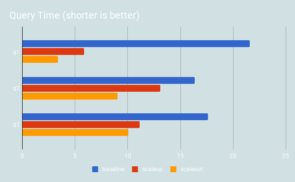
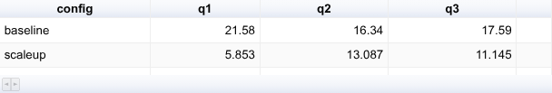
Following is a list of the queries, followed by a response time table recording the actual response times for each query. The queries should be self-explanatory.

Performance, at a glance

You will notice that Shard-Query is faster in nearly every case. The performance of the queries is improved significantly by scaling out, even more so than scaling up, because additional parallelism is added beyond what can be exploited by scale up. Scale up can improve query performance when there is enough resources to support the added parallelism, and when one of the the following are in used in the query: BETWEEN or IN clauses, subqueries in the FROM clause, UNION or UNION ALL clauses. If none of those features are used, then parallelism can’t be added. Q9 is an example of such a query.
.

Query details:

-- Q1<br> SELECT DayOfWeek, count(*) AS c<br>   from ontime_fact<br>   JOIN dim_date using (date_id)<br>  WHERE Year<br>BETWEEN 2000 AND 2008<br>  GROUP BY DayOfWeek<br>  ORDER BY c DESC;<br><br>-- Q2<br>SELECT DayOfWeek, count(*) AS c<br>  from ontime_fact<br>  JOIN dim_date using (date_id)<br> WHERE DepDelay&gt;10 AND Year BETWEEN 2000 AND 2008<br> GROUP BY DayOfWeek<br> ORDER BY c DESC;<br><br>-- Q3<br>SELECT CityName as Origin, count(*) AS c<br>  from ontime_fact<br>  JOIN dim_date using (date_id)<br>  JOIN dim_airport origin<br>    ON origin_airport_id = origin.airport_id<br> WHERE DepDelay&gt;10<br>   AND Year BETWEEN 2000 AND 2008<br> GROUP BY 1<br> ORDER BY c<br> LIMIT 10;

-- Q1 SELECT DayOfWeek, count(*) AS c from ontime_fact JOIN dim_date using (date_id) WHERE Year BETWEEN 2000 AND 2008 GROUP BY DayOfWeek ORDER BY c DESC; -- Q2 SELECT DayOfWeek, count(*) AS c from ontime_fact JOIN dim_date using (date_id) WHERE DepDelay>10 AND Year BETWEEN 2000 AND 2008 GROUP BY DayOfWeek ORDER BY c DESC; -- Q3 SELECT CityName as Origin, count(*) AS c from ontime_fact JOIN dim_date using (date_id) JOIN dim_airport origin ON origin_airport_id = origin.airport_id WHERE DepDelay>10 AND Year BETWEEN 2000 AND 2008 GROUP BY 1 ORDER BY c LIMIT 10;

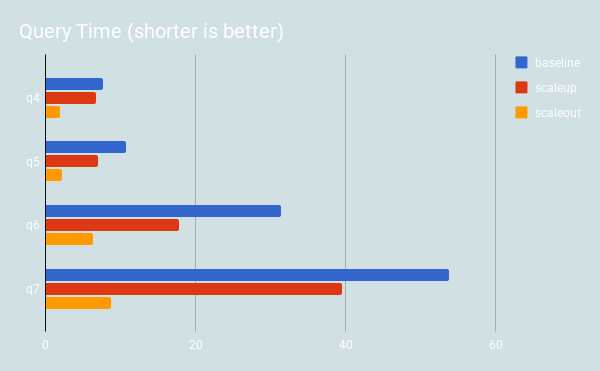
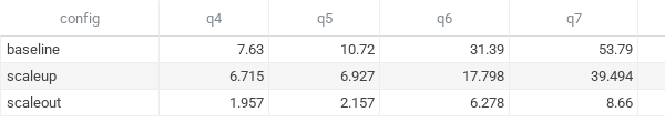
The next queries show how performance is improved when Shard-Query adds parallelism when “subqueries in the from clause” are used. There are benefits with both “scale-up” and “scale-out”, but once again, the “scale-out” results are the most striking.

-- Q4<br>SELECT Carrier, count(*) as c<br>  from ontime_fact<br>  JOIN dim_date using (date_id)<br>  join dim_flight using(flight_id)<br> WHERE DepDelay&gt;10<br>   AND Year=2007<br> GROUP BY Carrier<br> ORDER BY c DESC;<br><br>-- Q5<br>SELECT t.Carrier, c, c2, c*1000/c2 as c3<br>FROM<br>     (SELECT Carrier, count(*) AS c<br>        from ontime_fact<br>        join dim_date using(date_id)<br>        join dim_flight using(flight_id)<br>       WHERE DepDelay&gt;10<br>         AND Year=2007<br>       GROUP BY Carrier) t<br>JOIN (SELECT Carrier, count(*) AS c2<br>        from ontime_fact<br>        join dim_date using(date_id)<br>        join dim_flight using(flight_id)<br>       WHERE Year=2007<br>       GROUP BY Carrier) t2<br>  ON (t.Carrier=t2.Carrier)<br>ORDER BY c3 DESC;<br><br>-- Q6<br>SELECT t.Year, c1 / c2 as ratio<br>FROM<br>     (select Year, count(*)*1000 as c1<br>        from ontime_fact<br>        join dim_date using (date_id)<br>       WHERE DepDelay&gt;10<br>       GROUP BY Year) t<br>JOIN (select Year, count(*) as c2<br>        from ontime_fact<br>        join dim_date using (date_id)<br>       WHERE DepDelay&gt;10<br>       GROUP BY Year) t2<br>  ON (t.Year=t2.Year);<br><br>-- Q7<br>SELECT t.Year, c1 / c2 as ratio<br>  FROM (select Year, count(Year)*1000 as c1<br>          from ontime_fact<br>          join dim_date using (date_id)<br>         WHERE DepDelay&gt;10<br>         GROUP BY Year) t<br>  JOIN (select Year, count(*) as c2<br>          from ontime_fact<br>          join dim_date using (date_id)<br>         GROUP BY Year) t2<br>    ON (t.Year=t2.Year);

-- Q4 SELECT Carrier, count(*) as c from ontime_fact JOIN dim_date using (date_id) join dim_flight using(flight_id) WHERE DepDelay>10 AND Year=2007 GROUP BY Carrier ORDER BY c DESC; -- Q5 SELECT t.Carrier, c, c2, c*1000/c2 as c3 FROM (SELECT Carrier, count(*) AS c from ontime_fact join dim_date using(date_id) join dim_flight using(flight_id) WHERE DepDelay>10 AND Year=2007 GROUP BY Carrier) t JOIN (SELECT Carrier, count(*) AS c2 from ontime_fact join dim_date using(date_id) join dim_flight using(flight_id) WHERE Year=2007 GROUP BY Carrier) t2 ON (t.Carrier=t2.Carrier) ORDER BY c3 DESC; -- Q6 SELECT t.Year, c1 / c2 as ratio FROM (select Year, count(*)*1000 as c1 from ontime_fact join dim_date using (date_id) WHERE DepDelay>10 GROUP BY Year) t JOIN (select Year, count(*) as c2 from ontime_fact join dim_date using (date_id) WHERE DepDelay>10 GROUP BY Year) t2 ON (t.Year=t2.Year); -- Q7 SELECT t.Year, c1 / c2 as ratio FROM (select Year, count(Year)*1000 as c1 from ontime_fact join dim_date using (date_id) WHERE DepDelay>10 GROUP BY Year) t JOIN (select Year, count(*) as c2 from ontime_fact join dim_date using (date_id) GROUP BY Year) t2 ON (t.Year=t2.Year);

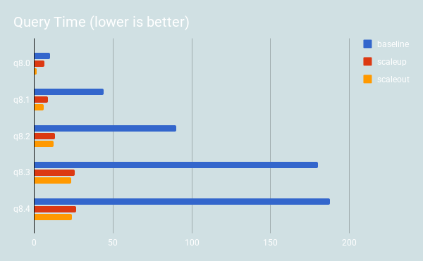
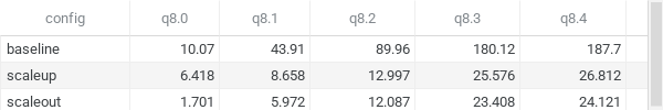
The performance of the following queries depends on the size of the date range:

-- Q8.0<br>SELECT dest.CityName, COUNT( DISTINCT origin.CityName)<br>  from ontime_fact<br>  JOIN dim_airport dest on ( dest_airport_id = dest.airport_id)<br>  JOIN dim_airport origin on ( origin_airport_id = origin.airport_id)<br>  JOIN dim_date using (date_id)<br> WHERE Year BETWEEN 2001 and 2001<br> GROUP BY dest.CityName<br> ORDER BY 2 DESC;<br><br>-- Q8.1<br>SELECT dest.CityName, COUNT( DISTINCT origin.CityName)<br>  from ontime_fact<br>  JOIN dim_airport dest on ( dest_airport_id = dest.airport_id)<br>  JOIN dim_airport origin on ( origin_airport_id = origin.airport_id)<br>  JOIN dim_date using (date_id)<br> WHERE Year BETWEEN 2001 and 2005<br> GROUP BY dest.CityName<br> ORDER BY 2 DESC;<br><br>-- Q8.2<br>SELECT dest.CityName, COUNT( DISTINCT origin.CityName)<br>  from ontime_fact<br>  JOIN dim_airport dest on ( dest_airport_id = dest.airport_id)<br>  JOIN dim_airport origin on ( origin_airport_id = origin.airport_id)<br>  JOIN dim_date using (date_id)<br> WHERE Year BETWEEN 2001 and 2011<br> GROUP BY dest.CityName<br> ORDER BY 2 DESC;<br><br>-- Q8.3<br>SELECT dest.CityName, COUNT( DISTINCT origin.CityName)<br>  from ontime_fact<br>  JOIN dim_airport dest on ( dest_airport_id = dest.airport_id)<br>  JOIN dim_airport origin on ( origin_airport_id = origin.airport_id)<br>  JOIN dim_date using (date_id)<br> WHERE Year BETWEEN 1990 and 2011<br> GROUP BY dest.CityName<br> ORDER BY 2 DESC;<br><br>-- Q8.4<br>SELECT dest.CityName, COUNT( DISTINCT origin.CityName)<br>  from ontime_fact<br>  JOIN dim_airport dest on ( dest_airport_id = dest.airport_id)<br>  JOIN dim_airport origin on ( origin_airport_id = origin.airport_id)<br>  JOIN dim_date using (date_id)<br> WHERE Year BETWEEN 1980 and 2011<br> GROUP BY dest.CityName<br> ORDER BY 2 DESC;<br>

-- Q8.0 SELECT dest.CityName, COUNT( DISTINCT origin.CityName) from ontime_fact JOIN dim_airport dest on ( dest_airport_id = dest.airport_id) JOIN dim_airport origin on ( origin_airport_id = origin.airport_id) JOIN dim_date using (date_id) WHERE Year BETWEEN 2001 and 2001 GROUP BY dest.CityName ORDER BY 2 DESC; -- Q8.1 SELECT dest.CityName, COUNT( DISTINCT origin.CityName) from ontime_fact JOIN dim_airport dest on ( dest_airport_id = dest.airport_id) JOIN dim_airport origin on ( origin_airport_id = origin.airport_id) JOIN dim_date using (date_id) WHERE Year BETWEEN 2001 and 2005 GROUP BY dest.CityName ORDER BY 2 DESC; -- Q8.2 SELECT dest.CityName, COUNT( DISTINCT origin.CityName) from ontime_fact JOIN dim_airport dest on ( dest_airport_id = dest.airport_id) JOIN dim_airport origin on ( origin_airport_id = origin.airport_id) JOIN dim_date using (date_id) WHERE Year BETWEEN 2001 and 2011 GROUP BY dest.CityName ORDER BY 2 DESC; -- Q8.3 SELECT dest.CityName, COUNT( DISTINCT origin.CityName) from ontime_fact JOIN dim_airport dest on ( dest_airport_id = dest.airport_id) JOIN dim_airport origin on ( origin_airport_id = origin.airport_id) JOIN dim_date using (date_id) WHERE Year BETWEEN 1990 and 2011 GROUP BY dest.CityName ORDER BY 2 DESC; -- Q8.4 SELECT dest.CityName, COUNT( DISTINCT origin.CityName) from ontime_fact JOIN dim_airport dest on ( dest_airport_id = dest.airport_id) JOIN dim_airport origin on ( origin_airport_id = origin.airport_id) JOIN dim_date using (date_id) WHERE Year BETWEEN 1980 and 2011 GROUP BY dest.CityName ORDER BY 2 DESC;

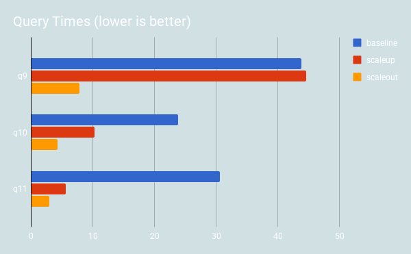
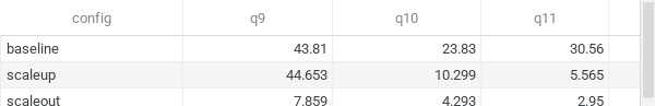
Finally, Shard-Query performance continues to improve when grouping and filtering is used. Again, notice Q9. It doesn’t use any features which Shard-Query can use to add parallelism. Thus, in the scale up configuration it does not perform any better than the baseline, and actually performed just a little worse. Since scale out splits the data between servers, it performs about 6x better as the degree of parallelism is controlled by the number of shards.

-- Q9<br>select Year ,count(Year) as c1<br>  from ontime_fact<br>  JOIN dim_date using (date_id)<br> group by Year;<br><br>-- Q10<br>SELECT Carrier, dest.CityName, COUNT( DISTINCT origin.CityName)<br>  from ontime_fact<br>  JOIN dim_airport dest on ( dest_airport_id = dest.airport_id)<br>  JOIN dim_airport origin on ( origin_airport_id = origin.airport_id)<br>  JOIN dim_date using (date_id)<br>  JOIN dim_flight using (flight_id)<br> WHERE Year BETWEEN 2009 and 2011<br> GROUP BY Carrier,dest.CityName<br> ORDER BY 3 DESC;<br><br>-- Q11<br>SELECT Year, Carrier, dest.CityName, COUNT( DISTINCT origin.CityName)<br>  from ontime_fact<br>  JOIN dim_airport dest on ( dest_airport_id = dest.airport_id)<br>  JOIN dim_airport origin on ( origin_airport_id = origin.airport_id)<br>  JOIN dim_date using (date_id)<br>  JOIN dim_flight using (flight_id)<br> WHERE Year BETWEEN 2000 and 2003<br>   AND Carrier = 'AA'<br> GROUP BY Year, Carrier,dest.CityName<br> ORDER BY 4 DESC;

-- Q9 select Year ,count(Year) as c1 from ontime_fact JOIN dim_date using (date_id) group by Year; -- Q10 SELECT Carrier, dest.CityName, COUNT( DISTINCT origin.CityName) from ontime_fact JOIN dim_airport dest on ( dest_airport_id = dest.airport_id) JOIN dim_airport origin on ( origin_airport_id = origin.airport_id) JOIN dim_date using (date_id) JOIN dim_flight using (flight_id) WHERE Year BETWEEN 2009 and 2011 GROUP BY Carrier,dest.CityName ORDER BY 3 DESC; -- Q11 SELECT Year, Carrier, dest.CityName, COUNT( DISTINCT origin.CityName) from ontime_fact JOIN dim_airport dest on ( dest_airport_id = dest.airport_id) JOIN dim_airport origin on ( origin_airport_id = origin.airport_id) JOIN dim_date using (date_id) JOIN dim_flight using (flight_id) WHERE Year BETWEEN 2000 and 2003 AND Carrier = 'AA' GROUP BY Year, Carrier,dest.CityName ORDER BY 4 DESC;

Conclusion

The divide and conquer approach is very useful when working with large quantities of data. Shard-Query can be used with existing data sets easily, improving the performance of queries significantly if they use common query features like BETWEEN or IN. It is also possible to spread your data over multiple machines, scaling out to improve query response times significantly.

These queries are a great test of Shard-Query features. It is currently approaching RC status. If you decide to test it and encounter issues, please file a bug on the bug tracker. You can get Shard-Query (currently in development release form as a checkout from SVN) here: Shard-Query Google code project

Full disclosure

Justin Swanhart, the author of this article is also the creator and maintainer of Shard-Query. The author has previously worked in cooperation with Infobright, including on benchmarking. These particular tests were performed independently of Infobright, without their knowledge or approval. Infobright was, however, given the chance to review this document before publication, as a courtesy. All findings are represented truthfully, transparently, and without any intended bias.