Ad-hoc Data Visualization and Machine Learning with mysqlshell

In this blog post, I am going to show how we can use mysqlshell to run ad-hoc data visualizations and use machine learning to predict new outcomes from the data.

Some time ago Oracle released MySQL Shell, a command line client to connect to MySQL using the X protocol. It allows us to use Python or JavaScript scripting capabilities. This unties us from the limitations of SQL, and the possibilities are infinite. It means that MySQL can not only read data from the tables, but also learn from it and predict new values from features never seen before.

Some disclaimers:

• This is not a post about to how to install mysqlshell or enable the X plugin. It should be already installed. Follow the first link if instructions are needed.
• The idea is to show some of the things that can be done from the shell. Don’t expect the best visualizations or a perfectly tuned Supervised Learning algorithm.

It is possible to start mysqlshell with JavaScript or Python interpreter. Since we are going to use Pandas, NumPy and Scikit, Python will be our choice. There is an incompatibility between mysqlshell and Python > 2.7.10 that gives an error when loading some external libraries, so make sure you use 2.7.10.

We’ll work the “employees” database that can be downloaded here. In order to make everything easier and avoid several lines of data parsing, I have created a new table that summarizes the data we are going to work with, generated using the following structure and query:

The data is:

• Age: the age of the employee
• Hired: the number of years working in the company
• Gender: 0 Male, 1 Female
• Salary: the salary 🙂

It only includes people currently working at the company.

Now that the data is ready, let’s start with mysqlshell. Everything that follows was done directly from the shell itself.

Starting the Shell and Loading the Libraries

Once the login is validated, we will see the following prompt:

That means we are using the shell in Python mode. We can start loading our libraries:

Now, we read each column from the table and store it in its own variable:

And create a Pandas dataframe used to generate the visualizations:

Data Analysis

Now, let’s investigate the data. Some basic statistics to get age, hired and salary overview:

Those statistics already give us good information. The employees range from 52 to 65, having an average of 59. They have been working at the company for 27 years on average with a salary of 72041.

But let’s forget about numbers. The human brain works much better and faster interpreting graphs than reading a table full of numbers. Let’s create some graphs and see if we can find any relationship.

Data Visualization

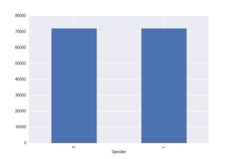
Relation between Gender and Salary:

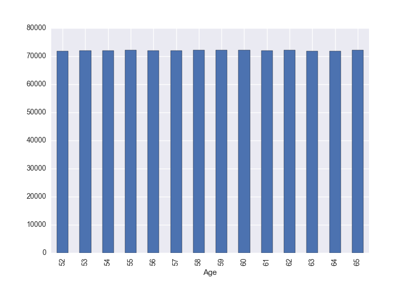
Relation between Age and Salary:

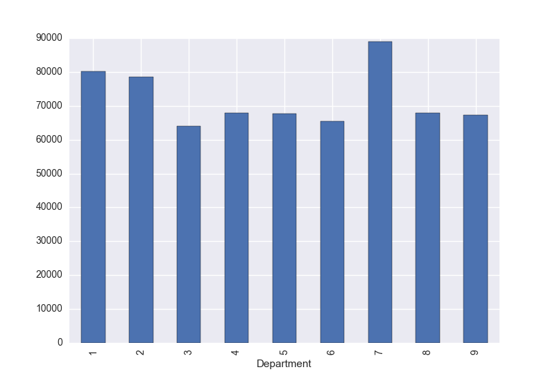
Relation between Department and Salary:

Relation between Hired and Salary:

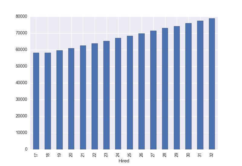
Now everything is more clear. There is no real relationship between gender and salary (yay!) or between age and salary. Seems that the average salary is related to the years that an employee has been working at the company, It also shows some differences depending on the department he/she belongs to.

Making Predictions: Machine Learning

Up to this point we have been using matplotlib, Pandas and NumPy to investigate and create graphs from the data stored in MySQL. Everything is from the shell itself. Amazing, eh? 🙂 Now let’s take a step forward. We are going to use machine learning so our MySQL client is not only able to read the data already stored, but also predict a salary.

Decision Tree Regression from SciKit Learn is the supervised learning algorithm we’ll use. Remember, everything is still from the shell!

Let’s separate the data into features and labels. From Wikipedia:

“Feature is an individual measurable property of a phenomenon being observed.”

Taking into account the graphs we saw before, “hired” and “department” are good features that could be used to predict the correct label (salary). In other words, we will train our Decision Tree by giving it “hired” and “department” data, along with their labels “salary”. The idea is that after the learning phase, we can ask it to predict a salary based on new “hired” and “department” data we provide. Let’s do it:

Separate the data in features and labels:

Train our decision tree:

Now, MySQL, tell me:

What do you think the salary of a person that has been working 25 years at the company, currently in department number 2, should be?

It predicts that the employee should have a salary of 75204. A person working there for 25 years, but in department number 7, should have a greater salary (based on the averages we saw before). What does our Decision Tree say?

Summary

Now MySQL can both read data we already know, and it can also predict it! 🙂 mysqlshell is a very powerful tool that can be used to help us in our data analysis tasks. We can calculate statistics, visualize graphs, use machine learning, etc. There are many things you might want to do with your data without leaving the MySQL Shell.